1. 策略梯度原理

在强化学习中，学习的目标是要找到一个策略 $\pi ^\ast$，使得总体回报的期望最高。这里的回报就是状态价值函数 $V^{\pi}\left ( s \right )$ 和动作价值函数 $Q^{\pi}\left ( s,a \right )$。而基于值的方法并不直接对策略 $\pi$ 建模，而是先学习并优化价值函数，然后基于价值函数来推导出最优策略：

$$\pi ^\ast \left ( s \right )=\underset{a}{argmax}\;Q^\ast\left ( s,a \right )$$

以上便是 value-based 强化学习的核心思想。

基于值的方法主要有三大类，分别为：动态规划、蒙特卡洛方法和时序差分算法。在动态规划中，需要事先知道转移矩阵 $P$ 和奖励函数 $r$，这两个参数就构成了模型，因此动态规划也划分到基于模型（model-based）方法。在无模型的方法中，蒙特卡洛方法的更新需要等到当前的采样结束后，才能对动作价值函数 $Q$ 更新，更新较慢，同时，蒙特卡洛方法的高方差也导致了整体的训练会出现不平稳的现象。在蒙特卡洛方法中，其更新公式为：

$$Q^{\pi }\left ( s_t,a_t \right ) \leftarrow Q^{\pi }\left ( s_t,a_t \right )+\frac{1}{N_{\left ( s_t,a_t \right )}}\left ( G- Q^{\pi }\left ( s_t,a_t \right ) \right )$$

基于时序差分算法对上述的问题进行了优化，典型的算法如 Sarsa 算法。在 Sarsa 算法中，由于其基于时序差分算法，能充分利用每一步来更新动作价值函数，其更新公式为：

$$Q^{\pi }\left ( s_t,a_t \right ) \leftarrow Q^{\pi }\left ( s_t,a_t \right )+\alpha \left ( R_t+\gamma Q^{\pi }\left ( s',a' \right )- Q^{\pi }\left ( s_t,a_t \right ) \right )$$

由于每一步的更新都依赖当前的策略 $\pi$，故 Sarsa 算法也被称之为 on-policy 的算法。

在 Sarsa 算法中，其学习的目标是在策略 $\pi$ 下的动作价值函数 $Q^{\pi }\left ( s_t,a_t \right )$，这是一个与当前策略 $\pi$ 相关的目标，在策略评估和策略更新时都是基于策略 $\pi$，而在 Q-Learning 算法中，其学习的目标是最优的动作价值函数 $Q^{\ast }\left ( s,a \right )$，其更新公式为：

$$Q^{\pi }\left ( s_t,a_t \right ) \leftarrow Q^{\pi }\left ( s_t,a_t \right )+\alpha \left ( R_t+\gamma \;\underset{a'}{max}Q^{\ast }\left ( s',a' \right )- Q^{\pi }\left ( s_t,a_t \right ) \right )$$

这个目标与策略无关，策略的评估和策略的更新不是同一个策略，因此 Q-Learning 算法也被称为 off-policy 算法。但是，在 Q-Learning 的实现过程中，包括以上的算法中，都需要维护一个动作价值函数的 Q-Table，其中，行表示的是状态，列表示的是动作，交叉处记录的是 Q 值。这样的一种环境，只能处理离散的问题，同时状态空间，动作空间都比较小的环境，然而现实世界中还存在着大量的连续型的环境。在这样的环境下，用表格存储所有状态是不现实的。

随后 Deep Q-Network 则是通过神经网络对 $Q\left ( s,a;\theta \right )$ 建模，解决了 Q-Table 的问题。

策略梯度方法则是抛弃对动作价值函数 $Q^{\pi}\left ( s,a \right )$ 的建模，而是根据概念，即强化学习的目标是要找到一个策略 $\pi _{\theta }$，使得总体回报的期望最高：

$$J\left ( \theta \right )=\textbf{E}_{\tau \sim \pi _{\theta}}\left [ R\left ( \tau \right ) \right ]$$

为了求 $J\left ( \theta \right )$ 的最大值，可以使用梯度上升：

$$\theta \leftarrow \theta +\alpha \nabla _{\theta }J\left ( \theta \right )$$

那么就是求 $\nabla _{\theta }J\left ( \theta \right )$：

$$\nabla _{\theta}J\left ( \theta \right )=\textbf{E}_{\tau \sim \pi _{\theta}}\left [ \sum_{t}\nabla _{\theta}log\;\pi _{\theta }\left ( a_t\mid s_t \right )G\left ( t \right ) \right ]$$

其中：

$$G_t=\sum_{k=t}^{\infty }\gamma ^{k-t}r_k$$

2. REINFORCE

2.1. 算法原理

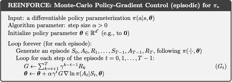
REINFORCE^[1] 是最经典、最基础的 Policy Gradient（策略梯度）算法，由 Ronald J. Williams (1992) 提出。在策略梯度原理中，要估计期望，REINFORCE 中是使用多次采样回报的方式估计回报的梯度的，简单来说就是：

$$\nabla _{\theta}J\left ( \theta \right )\approx \frac{1}{N}\sum_{i=1}^{N}\sum_{t=0}^{T_i-1} \nabla _{\theta}log\;\pi _{\theta }\left ( a^{\left ( i \right )}_t\mid s^{\left ( i \right )}_t \right )G^{\left ( i \right )}\left ( t \right )$$

REINFORCE 算法的整个过程^[2]：

2.2. 算法实现

采用的环境是 Cart Pole^[3]，这是一个连续状态的问题。该问题的动作空间中的动作有两个，状态是由 4 个值确定的，分别为 Cart Position，Cart Velocity，Pole Angle 和 Pole Angular Velocity。更多详细情况如参考文献 3。

2.2.1. 构建网络

首先，需要创建一个策略网络，以最简单的三层 DNN 网络为例，构建 PolicyNetwork 类：

# INFO: 策略网络
class PolicyNetwork(nn.Module):
    def __init__(self, n_observations, n_actions, hidden_dim=128):
        super(PolicyNetwork, self).__init__()
        self.fc1 = nn.Linear(n_observations, hidden_dim)
        self.fc2 = nn.Linear(hidden_dim, hidden_dim)
        self.fc3 = nn.Linear(hidden_dim, n_actions)

    def forward(self, x):
        x = F.relu(self.fc1(x))
        x = F.relu(self.fc2(x))
        x = self.fc3(x)
        return F.softmax(x, dim=-1)   # 输出动作概率分布

2.2.2. 训练

有了以上的结构的准备，接下来就是要按照上述的训练流程，实施“采样->更新”这样的循环，直接上代码：

class REINFORCEAgent:
    def __init__(self, env, device):
        self.env = env
        self.device = device

        self.n_actions = env.action_space.n
        self.n_observations = env.observation_space.shape[0] # 连续空间

        # INFO: 策略网络
        self.policy_net = PolicyNetwork(self.n_observations, self.n_actions)

        self.lr = 3e-4 # 学习率
        self.optimizer = optim.AdamW(self.policy_net.parameters(), lr=self.lr, amsgrad=True)
        self.scheduler = StepLR(self.optimizer, step_size=100, gamma=0.95)

        # INFO: 其他参数
        self.gamma = 0.99
        self.num_episodes = 2000

    def __update_policy(self, saved_log_probs, saved_rewards):
        # INFO: 统计回报
        G = 0
        discounted_rewards = []
        for reward in reversed(saved_rewards):
            G = reward + self.gamma * G
            discounted_rewards.insert(0, G)
        # 归一化（可选，有助于稳定训练）
        discounted_rewards = torch.tensor(discounted_rewards)
        discounted_rewards = (discounted_rewards - discounted_rewards.mean()) / (discounted_rewards.std() + 1e-9)

        policy_loss = []
        for log_prob, G_t in zip(saved_log_probs, discounted_rewards):
            # 损失 = - log_prob * G_t   (梯度上升转换为梯度下降)
            policy_loss.append(-log_prob * G_t)
        self.optimizer.zero_grad()
        policy_loss = torch.cat(policy_loss).sum()
        ret_loss = policy_loss.item()
        policy_loss.backward()
        self.optimizer.step()
        return ret_loss

    def train(self):
        episode_rewards = []
        train_loss = []
        for episode in range(self.num_episodes):
            # INFO: 1. 模拟采样
            state, _ = self.env.reset() # 重置环境
            state = torch.tensor(state, dtype=torch.float32, device=self.device).unsqueeze(0)
            episode_reward = 0
            done = False
            # INFO: 策略更新的两个参数
            saved_log_probs = []
            saved_rewards = []
            while not done:
                # INFO: 选择动作
                probs = self.policy_net(state)
                m = torch.distributions.Categorical(probs=probs)
                action = m.sample()
                saved_log_probs.append(m.log_prob(action))

                # INFO: 执行动作
                observation, reward, terminated, truncated, _ = self.env.step(action.item())
                done = terminated or truncated

                if terminated:
                    next_state = None
                else:
                    next_state = torch.tensor(observation, dtype=torch.float32, device=self.device).unsqueeze(0)
                
                saved_rewards.append(reward)
                
                episode_reward += reward
                state = next_state

            # INFO: 2. 策略更新
            ret_loss = self.__update_policy(saved_log_probs, saved_rewards)
            episode_rewards.append(episode_reward)
            train_loss.append(ret_loss)
            self.scheduler.step()

            if (episode+1) % 100 == 0:
                avg_reward = np.mean(episode_rewards[-100:])
                print(f"Episode {episode+1}, Average Reward (last 100): {avg_reward:.2f}")
        
        # INFO: 最终保存出模型
        torch.save(self.policy_net.state_dict(), 'reinforce_cartpole.pth')

        # INFO: 保存最终的训练状态
        fig, (ax1, ax2) = plt.subplots(1, 2, figsize=(8, 4))  # 1行2列，图形尺寸可调

        ax1.plot(episode_rewards)
        ax1.set_xlabel("episode")
        ax1.set_ylabel('reward')
        ax1.set_title('Reward')

        ax2.plot(train_loss)
        ax2.set_xlabel("epoch")
        ax2.set_ylabel('loss')
        ax2.set_title('loss')

        plt.tight_layout()
        plt.savefig("reward_loss.png")

有了完整的过程，启动训练：

if __name__ == "__main__":
    device = torch.device("cuda" if torch.cuda.is_available() else"cpu")
    env = gym.make("CartPole-v1")
    reinforce_agent = REINFORCEAgent(env, device=device)
    reinforce_agent.train()
    env.close()

2.2.3. 结果与测试

经过简单的训练，最终保存出名为 reinforce_cartpole.pth 目标网络的模型，同时我们可以看到训练过程中的数据表现：

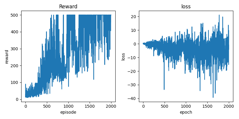
注：在 REINFORCE 算法中，loss 出现正负不断跳动的情况，这是正常情况，因为 $G_t$ 可正可负。

再写一段测试的脚本，用于测试模型的表现，如下：

if __name__ == "__main__":
    mode = "test"
    device = torch.device("cuda" if torch.cuda.is_available() else"cpu")
    if mode == "train":
        env = gym.make("CartPole-v1")
        reinforce_agent = REINFORCEAgent(env, device=device)
        reinforce_agent.train()
        env.close()
    else:
        test_env = gym.make("CartPole-v1", render_mode='human')
        n_actions = test_env.action_space.n
        n_observations = test_env.observation_space.shape[0] # 连续空间
        # INFO: 定义模型
        policy_net = PolicyNetwork(n_observations, n_actions).to(device)
        # 2. 加载状态字典
        state_dict = torch.load('reinforce_cartpole.pth', map_location=torch.device('cpu'))  # 或 'cuda'

        # 3. 将参数加载到模型中
        policy_net.load_state_dict(state_dict)

        # 4. 设置为评估模式（如果只做推理）
        policy_net.eval()

        num_episodes = 10

        for ep in range(num_episodes):
            state, _ = test_env.reset()
            done = False
            total_reward = 0
            while not done:
                test_env.render()

                state = torch.tensor(state, dtype=torch.float32, device=device)
                probs = policy_net(state)
                m = torch.distributions.Categorical(probs=probs)
                action = m.sample()

                next_state, reward, terminated, truncated, _ = test_env.step(action.item())
                done = terminated or truncated
                total_reward += reward
                if done:
                    print(f"terminated: {terminated}, truncated: {truncated}")
                    break
                state = next_state
            print(f"Test Episode {ep+1}: Total Reward = {total_reward}")
        test_env.close()

3. 总结

REINFORCE 算法是最经典、最基础的 Policy Gradient（策略梯度）算法，由 Ronald J. Williams (1992) 提出，直接对策略建模，寻找到最优的策略使得总体回报的期望最高。从实验的结果来看，与 DQN 相比，效果及稳定性要低于 DQN。

参考文献

[1] Williams R J. Simple statistical gradient-following algorithms for connectionist reinforcement learning[J]. Machine learning, 1992, 8(3): 229-256.

[2] http://incompleteideas.net/book/RLbook2020.pdf

[3] https://gymnasium.farama.org/environments/classic_control/cart_pole/